Results
Results
import os
import pandas as pd
import matplotlib
import seaborn as sns
import matplotlib.pyplot as plt

df_data = pd.read_csv(os.path.join('..', '..', '..', 'resources', "compressed_images.csv"))

df_data.head()
| subjectID | site | age | gender | df_comp_1 | gm_comp_1 | wm_comp_1 | csf_comp_1 | df_comp_2 | gm_comp_2 | wm_comp_2 | csf_comp_2 | |
|---|---|---|---|---|---|---|---|---|---|---|---|---|
| 0 | sub-256 | HH | 27.38 | 0 | -1.299959 | 1.493881 | 2.118407 | -1.402236 | 0.983905 | -1.425386 | -0.569065 | 0.620575 |
| 1 | sub-332 | IOP | 42.37 | 1 | 0.094058 | -0.395575 | -1.058985 | 0.283817 | -1.981011 | 0.442281 | -0.075717 | -1.461559 |
| 2 | sub-541 | IOP | 36.42 | 1 | -0.742552 | 0.325113 | -0.772167 | -1.127778 | -0.817974 | -0.406767 | -0.788280 | 0.098370 |
| 3 | sub-043 | Guys | 22.65 | 1 | -1.015449 | 1.357072 | -0.715433 | -1.518454 | 1.500735 | -1.607872 | -1.068050 | 1.333944 |
| 4 | sub-022 | Guys | 30.67 | 0 | 0.344976 | 1.282205 | 1.484323 | 1.181775 | 0.801336 | 1.847277 | -0.994154 | 0.239034 |
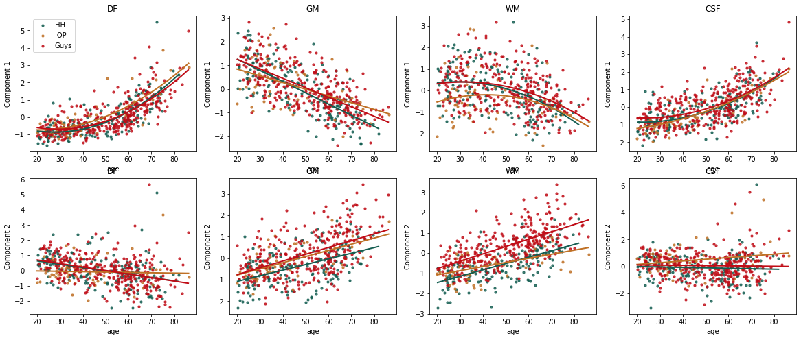
effect = "site"

order_mod = {"df": [2, 1], "gm": [1, 1], "wm": [2, 1], "csf": [2, 1]}

n_comps = 2
n_col = len(order_mod)
total_display = n_col*n_comps

n_rows = int(total_display/n_col)


color_palette = ["#135D50", "#BF7025", "#C00C16"]

f = plt.figure(figsize=(5*n_col, 4*n_rows))
f.tight_layout()
for comp in range(n_comps):
    for i, ext in enumerate(order_mod):

        f.add_subplot(n_rows, n_col, n_col*comp+i+1)
        for k, effect_i in enumerate(df_data[effect].unique()):
            sns.regplot(data=df_data.loc[df_data[effect] == effect_i], x = 'age', y = f'{ext}_comp_{comp+1}', color=color_palette[k],
                        order=order_mod[ext][comp], label=effect_i, ci=None, scatter_kws={'s':10}, line_kws={'linewidth':2})
        plt.title(f'{ext.upper()}')
        plt.ylabel(f'Component {comp+1}')
        plt.ticklabel_format(axis='y', scilimits=(0, 0))

        if comp != 0 or i != 0:
            plt.legend().remove()
        else:
            plt.legend()